Statistics Review

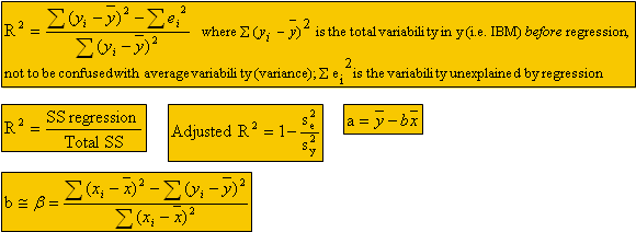
Random variable – variable that takes on numerical values determined by the outcome of a random experiment. Usually denoted by X
Probability distribution – expresses probability that a continuous random variable takes on value X=x

• Adding a constant to a variable shifts the distribution
• Multiplying by a constant changes the dispersion of a variable (if <1σ reduces, if >1σ increases)

To compute the probability for a normal random variable, convert X~N(μ, σ²) to Z~N(μ, σ²):

Point Prediction – If data is independent, the best prediction is the mean. If data is not independent (runs test significant at <0.05) then X_t+1 = X_t + μ_change + ε_t

Runs Test

• Few runs -> cyclical time series
• Many runs -> oscillating time series
• Medium # of runs -> independent time series
• When we predict for independent series (=μ of series) the confidence interval is a multiple of σ
• When we predict for non-independent time series (=μ_change + ε_t) the confidence interval is a multiple of the variance (σ²) {e.g. X₇₀ ~ N(X₆₈ + 2μ_change , 2σ_change²)}

A random walk exists is the changes from period to period are independent and normally distributed

Estimating μ and σ {X representative of μ, s² representative of σ²)

• If X ~ N(μ, σ²) then X  ~ N(μ, σ²/n)

Linear Regression (α + ßx) + ε_t with ε_t iid N(μ, σ_ε²)
Make distance from each point to the estimated line as small as possible. Minimize Σε_t²

4 Basic Assumptions and how to check them:

• linearity – non-linear pattern in x/y plot; u-shaped pattern in the Residuals vs. Fit plot
• constant variance – look for funnel in the Residuals vs. Fit plot
• independence – pattern in time series plot; runs test
• normality – histogram of e’s (residual = e)

Assuming X is independent (data set) implies the e’s are independent. Must check this.

Specification bias – exists when an explanatory variable that should be included in regression is left out. {if a coefficient doesn’t make sense it could be due to specification bias}

Understanding the Regression Output:

In regressions, error terms don’t accumulate (predictions)
Coefficients are random variables because they depend on sample of points
Any time you standardize using an estimate you get a t-distribution not a z-distribution

• Dummy variables are useful when the # of data points isn’t sufficient for multiple single regressions
• Interpret regression model using dummy variables as multiple parallel regression lines where the coefficients are the distance between the lines
• Baseline is the dummy variable that is left out (intentionally) when running the regression
• Best prediction of true regression α +  ßx = ε is a + bx (ε=0)

Confidence Intervals
2 components of prediction error:

1. (α +  ßx) – (a + bx)
2. ε
   • the ore uncertainty about the 2 sources of error, the more uncertain the prediction is and therefore a wider confidence interval
   • Minitab gives a 95% interval

Time Series with Trend
Pattern consists of:

• Trend – model with Time variable
• Seasonal component – model with multiple dummy variables
• Short-term correlation (cyclical) – model w/ Y_t-1
• Unpredictable component (ε)

To modify the model to account for non-constant variance, run a regression model for % change in variable (i.e. sales) {this is like a non-independent time-series point prediction}

Leading indicators can improve the model BUT are not useful for predicting

It is important to know how close b is to ß:
The sampling distribution for b is b ~ N(ß, σ_b²)     

Hypothesis Testing:  (H₀: ß=0  H_A: ß<>0) – useful for determining which variables have explanatory power
Type I Error – say ß=1 when ß=0 (reject H₀ when H₀ is true)
Type II Error – say ß=0 when ß=1 (accept H₀ when H₀ is false)

Procedure:

1. Collect sample
2. Compute b
3. Compare to critical t-value
4. Reject H₀ if (b/s_b) > t_critical

We’re choosing a cutoff value such that pr(Type I error) = 0.05 (α)
Each coefficient has a t-distribution with (n – total # coefficients) degrees of freedom (t_n-#, _α)

• If one-sided decision (i.e. H_A: ß>0), use α as given percentage
• If two-sided decision (i.e. H_A: ß>0), use α as ½ of the given percentage