MacroEconomics Review

Aggregate Price Level (P) – average price of goods and services in the economy measured by CPI or GNP Deflator

Financial intermediaries/markets – address imperfections in markets (risk, liquidity, search costs, economies of scale) and help avoid adverse selection – unequal (asymmetric) info before a transaction; and moral hazard – incentive to one party after the transaction to undermine value to other party.

Reasons for regulation:

1. Increase information to investors
2. Ensure soundness of financial intermediaries
3. Improve monetary control

Asset – store of value; something that will provide future benefits.

Wealth elasticity of (asset) demand = % change demanded / % change in wealth

• Necessity – wealth elasticity < 1 {lower risk or conservative asset}
• Luxury – wealth elasticity > 1 {higher risk or aggressive asset}

Ceteris Paribus – everything else equal.

Fisher Effect – when expected inflation rises, interest rates rise (i_n=i_r + π^e)

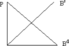
Bonds (classical curve)

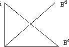
Bonds (as viewed by an individual)

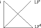
Loanable Funds (as viewed by a corporation)

liquidity preference framework (Keynes) – determines equilibrium i in terms of Money supply and demand
loanable funds framework – determines equilibrium i in terms of supply and demand of bonds

loanable funds framework is easier to use with respect to changes in expected inflation π^e; liquidity preference framework is easier to use with respect to changes in income, price level and supply of money.

Keynes – 2 categories of assets people use to store wealth:

1. Money
2. Bonds

M^s + B^s = wealth ⇒ B^d + M^d = wealth ⇒ M^s + B^s = B^d + M^d ⇒ M^s – M^d = B^d – B^s

* liquidity preference framework ignores effects from changes in expected returns on real assets; Keynes assumed i=0 for money.

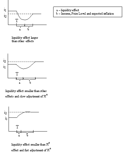
liquidity effect – lowering of interest rate due to increase of M^s (Milton Friedman)

3 reasons people hold money:

1. transaction motive = f(y) {y = GNP (income)}
2. precautionary motive = f(y)
3. speculative motive = f(i)

* A change in price level is an after-the-fact effect not an effect of expectation:
income ↑ ⇒ Price ↑ (employees scarce ⇒ wages ⇒ prices to consumer ↑)

Effects of money on interest rates:

• liquidity effect: M^s ↑ ⇒ i ↓ (spurs economic activity, expansion)
• income effect: M^s ↑ ⇒ income ↑ ⇒ M^d ↑⇒ i ↑
• price level effect: M^s ↑ ⇒ P ↑ ⇒ i ↑
• π^e effect: M^s ↑ ⇒ π^e ↑ ⇒ B^d ↓, B^s ↑ ⇒ i ↑

risk premium – i_corp – i_treasury
{risk structure – bonds of same maturity; term structure – bonds of diff. maturity}

Factors affecting bond ratings:

• firm’s financial condition
• industry environment
• regulatory constraints

*risk premium reflects corporate bonds lower liquidity in addition to default risk

Term structure facts to be explained:

1. interest rates for different maturities move together
2. yield curves have steep slope when short rates are low, down slope when short rates are high
3. yield curve typically upward sloping

3 theories to explain term structure attributes:

1. expectations hypothesis – bonds of different maturities are perfect substitutes, so i for long-term bond = average of short-term rates expected over life of long-term bond.
2. segmented markets – bonds of different maturity not perfect substitutes; explains typical upward slope but not other 2 attributes.
3. preferred habitat theory – interest rate on long-term bond = average of short-term rates + term premium that responds to demand and supply for that bond

Yield Curves

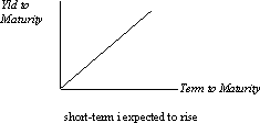
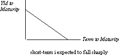
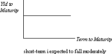
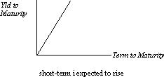
we can use yield curves to tell what the market is predicting for future short-term rates.

Term Structure: Forward Rates


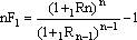
{forward rate = short-term rate for future bond}

Exchange Rates:
A stronger dollar leads to less expensive foreign goods and more expensive U.S. goods exported abroad.